For clinicians, understanding the diagnostic accuracy of the tests we order is vital. Often, test results are continuous, necessitating a dichotomous categorization into ‘disease present’ or ‘disease absent’. This decision hinges on setting an appropriate cut-off value at which we call the test a ‘positive’ result. The Receiver Operating Characteristic (ROC) curve is a fundamental tool to visualize the trade off between sensitivity and specificity at different thresholds of test positivity.
The Basics: Sensitivity, Specificity, and the Decision Matrix
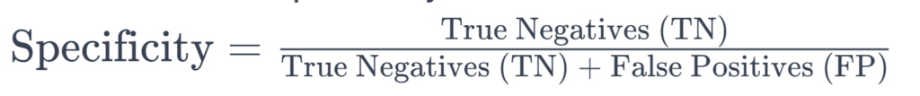
To grasp ROC curves, we first need to understand sensitivity and specificity. Sensitivity measures the proportion of actual disease cases correctly identified by the test while specificity refers to the correct identification of non-disease cases (see formulas below). A perfect test would have a sensitivity and specificity of 1.0 (or 100%) but this does not occur in the real world.

What is an ROC Curve?
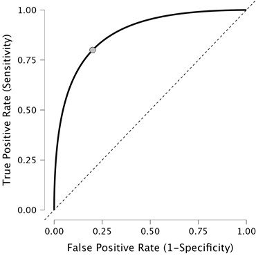
The ROC curve, developed during World War II for signal detection, now serves as a key tool in medical diagnostics. It plots sensitivity (true positive rate) against 1 – specificity (false positive rate) for various cut-off values of a test, helping to identify the optimal balance between sensitivity and specificity.
Types of ROC curves
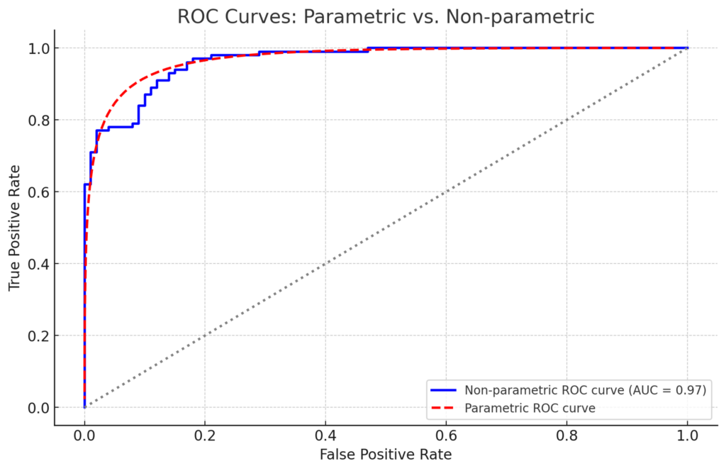
ROC curves are either nonparametric (empirical) or parametric. The nonparametric ROC curve, commonly used in medicine, does not assume a specific distribution of test results and appears as a jagged line. The parametric curve, smoother in appearance, assumes a normal distribution of test results.
Drawing a ROC curve
Consider a scenario with ten patients undergoing a cancer marker test. As the cut-off value to determine whether the patient has cancer is adjusted, the sensitivity and specificity vary, allowing the plotting of these points on a graph. For example, we could make the test very sensitive and have very few false negatives, but this might come at the expense of false positives. The resulting curve helps visualize the trade-off between sensitivity and specificity.
The importance of AUC (area under the curve)
AUC quantifies the overall accuracy of a diagnostic test. An AUC of 1.0 signifies a perfect test, while an AUC of 0.5 indicates no diagnostic utility. Generally, an AUC above 0.8 is deemed acceptable for a diagnostic test, but this varies depending on the role of the test in the clinical pathway.
| Area under the Curve (AUC) | Interpretation |
|---|---|
| 0.9 ≤ AUC | Excellent |
| 0.8 ≤ AUC < 0.9 | Good |
| 0.7 ≤ AUC < 0.8 | Fair |
| 0.5 ≤ AUC < 0.7 | Poor |
| AUC < 0.5 | Unacceptable |
Determining the Optimal Cut-off Value
The optimal cut-off value is not merely about maximizing sensitivity and specificity but finding a suitable balance based on the clinical context. Various methods, such as Youden’s J statistic, Euclidean distance, and cost approaches, help in determining this value.
Statistical Programs for ROC Analysis
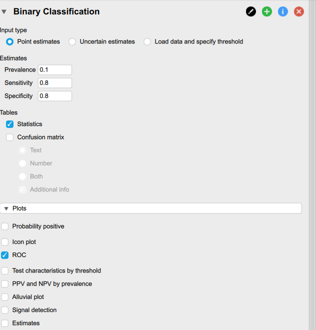
Various commercial programs (R, SPSS) exist to generate ROC curves. I recommend using the free software JASP which is super simple to use – you can just put in the values and automatically generate curves. No programming required!
Conclusion
ROC curves are helpful for clinicians to understand the tradeoff between sensitivity and specificity for different test positivity thresholds. The AUC is a valuable test metric that encompasses the overall accuracy of the test.
Wanting to learn more about research methods? Continue reading about what a P-value is (and what a P-value is not!)